2020 Vision & Goals

I’ve been a bit inactive of late, a combination of getting a new machine learning computer and work. Still, it’s given me time have a rethink about my approach to generating new Grateful Dead audio.

I have two new approaches I want to try out this year. You could say one of them has already been done – that is, someone has already generated “fake Grateful Dead” audio, and you’ve listened to it and accepted it as the real thing for years!

Filling In The Gaps

Some older shows recorded on digital (typically early 80’s shows) can suffer from digi-noise, that is, pops and hiccups caused by the tape simply being a little old and losing some of it’s digital information. for a (really bad) example of this, see https://archive.org/details/gd1981-09-25.sbd.miller.88822.sbeok.flac16 (and check out the weird split Sugar Mag if you can get past the sound issues).

Not all tapes are this bad, and in fact in most cases when this happens someone like Charlie Miller will cover up the noise with some editing. But think about that sentence again: “cover up the noise with some editing”, hey that sounds like putting in fake audio. You have a piece of music with a discontinuity, and you have to fill it with something that sounds nicer and sounds like the GD, right?

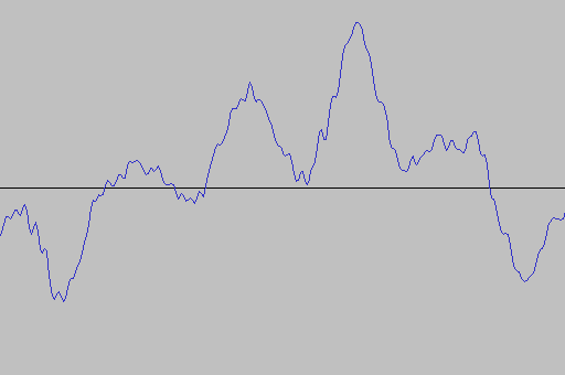
Well, almost. Look at a typical sample of digi-noise:

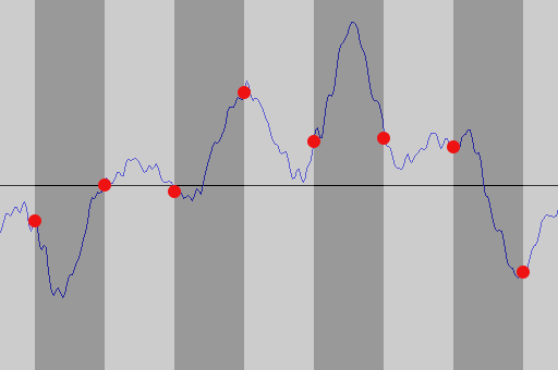
This digi-noise would be pretty loud compared with the rest of the audio (which is why we want to hide it). However, if we zoom in:

We can see that in fact the time for this audio event is from ~3.0195s to 3.0226, i.e. 0.0031s. That’s just 3/100’s of a second, which is probably easy enough to fix in a studio.

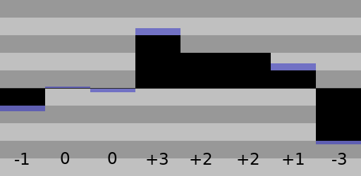
But this problem is ideal for generating new GD audio. Up to now, my effort has been to “teach” the computer by feeding it a large amount of GD, and then asking it to make some original audio. The problem with this approach is that the test is very difficult for the computer. If I first asked you to read every single Stephen King novel and then tasked you with writing a new paragraph in the same style, you would find that difficult. If however I asked you to start by filling in a missing word, well that would be a lot easier. Or if that was too much, start with a single letter.

And that, in a nutshell, is the new approach. Instead of asking the computer to generate new audio from scratch, we instead ask it to fill in the missing audio. At first this will be someting like 3/100ths of a second. When that works, I simply ask it to fill it larger and larger gaps.

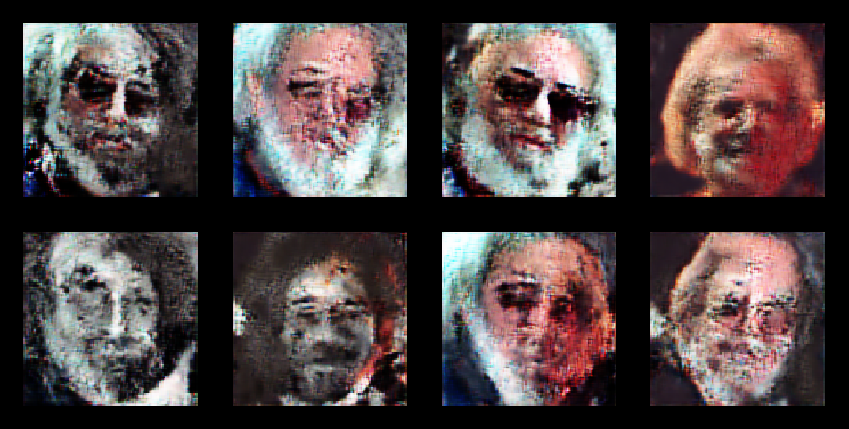
This approach has been tried for images, and the results are pretty good.

GANS network filling in image after training on human faces

As you can see, the computer is able to generate many images to fill in the blank space.

Style Transfer

The second thing I shall try this year is a “style-transfer” with GD audio. These are best explained with images. Example: I have some photos. I also have digital copies of many paintings. I train the computer to recognise the style of the painter and “transfer” my image into the style of the painter.

Basic image on left, styles applied on right

So what styles are there in GD audio? Of all the tapes I have ever listened to, they are almost always one of two styles: audience or soundboard. So I will train the computer to tell the difference between them, and then ask it to output the audience audio into the style of a soundboard. I hasten to add that quite a few people prefer audience tapes (especially with the somewhat dry soundboard tapes of the early 80s), and that the style could easily go the other way.

Time Dependency

This last point is a technical issue, but one which could offer easily the best results.

So, a sound file is – to the computer – a linear series of numbers (each number being the volume at a given point in time).

What we are really asking the machine to do is to continue generating a series of new numbers based on the numbers so far.

But think how you might do this. To accurately guess what comes next, we work on a number of differing timescales. Note in the scale? Chord in the sequence? Verse to be sung? Is it a Bobby number next? All my attempts so far have been really concentrating on the “next note”, because music generates a lot of audio and so we only want to really check the local time area otherwise our computation gets really slow. In effect, to generate the next second of music, my code so far only looks at the previous 2-4 seconds. But to produce longer samples, we will need the computer to understand a lot more about the structure of the song.

I don’t want to get super-technical here, but Google researchers have a partial solution to this, which they used for creating realistic human voices (paper here: https://arxiv.org/abs/1609.03499).

It essentially means my software will be able to take inferences from a much much larger area of the song. Generating a longer section of audio might not get any quicker but no longer will the computer have the memory of a goldfish. I’m really interested in this approach because it’s been tried and tested. Here, for example, is a section of music generated by a computer that has been trained on piano recitals.

Piano recital sample generated purely from the mind of a computer

My point being: If it can be done with piano recitals, it can be done with the Grateful Dead.

Finally, Results

Yes. you read that headline correctly: I have results! However, those expecting authentic sounding Grateful Dead – in whatever form that may take – will probably want to be waiting a lot longer. But if we view this whole process as akin to cooking a meal, I have at least sorted out the ingredients and cutlery, even if the food so far is somewhat lacking.

Again, our friend phase

So the basic approach was as outlined in the previous blog post. We build 2 computer programs, 1 to detect Grateful Dead music and the other to create some music. Then we put these 2 machines in an evolutionary arms race, as they should slowly get better at their jobs, and ultimately the generator should be able to create new Grateful Dead music (or at least, new music that you cannot tell is different).

The approach taken is not to use actual music (because this is difficult), but instead to do some processing on the sound beforehand. We actually split the audio into hundreds of time slices, and then work out all the sine waves of each slice. Since this is the format we input, it is also the format we output.

This gives us a problem with the output. Let’s imagine a piece of audio composed of 2 sine waves. It would look like this:

2 sine waves, representing a single sound

You can see that the starting point for both of these sine waves – the left hand side of the graph – is different. The red sine wave starts high up and the blue low down. This information is known as the phase of the signal.

The problem our generator has is that it generates sine waves but no phase information. Our generator then starts all sine waves at point 0 – the black line. But is has to do this for all the times we slice the audio up. The result is a set of broken sine waves, where the wave is “reset” at the start of every time slice:

Audio file with phase=0 at start of every timeslice

As you can see, this is most definitely not going to sound like what we want!

Simple solutions for the win

I really took some time to try and fix this issue. It is a known problem in audio processing and basically there is no fix for this. There have been some attempts using machine learning, but that would involve another huge amount of work. so instead, I did something very simple and it seemed to work. Quite simply, I just randomised the phase information, instead of setting it to 0 all the time. As can been in the diagram above, there is a repetition in the phase information at the start of every time step. This repetition really sticks in the ear. If you randomise the phase information, then you get something more like this:

Phase at every time stamp randomised instead of constant zero

This is not perfect, but now the results sound a lot better, and phase randomisation turned out to be not that hard to implement. With that out of the way, let’s move on to the results.

What we don’t expect

So essentially, the computer code is trying to replicate a certain style of music. If it were unable to incrementally get better, we might expect it to just produce random noise. In particular, we might expect white noise.

3 second sample of white noise

Or even pink noise, which is apparently what the sound crew used to test the GD’s audio system before a gig (pink noise is where the volume of the differing sound waves is equal):

3 second sample of pink noise

So for any success, we do don’t want to sound like these 2. What we do want is sound like the Grateful Dead. So here is a sample of the Grateful Dead in exactly the same format as my results – a 22050Hz mono audio sample:

Bonus points for guessing year, show or song!

The Results

After many hours of rendering audio, my program produced some samples. To the best of my knowledge, this is the first computationally created Grateful Dead audio to ever be generated (more epochs should be better):

Render after 1000 epochs

Render after 1500 epochs

Render after 2000 epochs

So – is this progress? It is certainly not the Grateful Dead, but on the other hand it is not white or pink noise. It is also – unlike my previous posts – actual audio. I count this as a partial success, but also an indicator the final goal is some distance away.

The Future

The obvious thing to do now is to increase everything – the amount of music I use as data, the length of time I spend processing, and the size of the output data. This will take some time. I have another approach up my sleeve that involves generating songs from a very low resolution and then increasing the resolution, as opposed to starting with a small piece of music and trying to make it longer. But that’s for another post!

Finally Getting The Data Right

I’ve been a bit quiet in posting recently, not such for a lack of work, more a lack of progress. But this weekend I did indeed finally mange to get my data sorted.

Those of you following along so far may know that I’ve had difficulty with my data format, that is, the stuff I actually give to the computer to learn from. There are 2 ways of doing things. I can use a Mel spectrogram – which is a mathematical conversion of sound into an image – or I could use a normal uncompressed wav file.

The MEL way seemed good because, on the face of it,, I managed to get the whole process working. I was able to train a Grateful Dead discriminator, followed by a producer that seemed to put out pretty good MEL representations. Here was new Grateful Dead music! To remind ourselves, I got this:

Real Grateful Dead audio on the left: machine learnt audio on the right

But…. you can’t hear a MEL image, can you? These couldn’t be converted into sound. With wav files, the exact opposite problem: turning them into sound is trivial, but I couldn’t get the machine learning actually learning at all (a common problem with wavs in the ML world). Over this the summer I tried various ways for the wav method to work, but it never did. It became obvious that I had to go the MEL route since it actually worked. This meant turning a MEL image back into audio, and that in turn meant tackling the maths.

Anatomy of a MEL

So how is a MEL made? The first step is the hardest to understand, although it is easy enough to express. We use a Fourier transform (some fancy maths) to take some sound and decompose it into its constituent frequencies. Give it some audio and you end up with a collection of sine waves. We don’t do this for the entire audio – we do one Fourier transform for every 1/5th of a second, as an example, so ending up with a series of time blocks for which we have all the sine waves generated by the band in that time period.

The final stage is to adjust this so that the frequencies we hear in our ears are increased in power, and those that the ear finds harder to hear, we diminish. We want the machine to “hear” the same that we do (this is actually the “MEL” part of “MEL Spectrogram”.

The Hard Work

When I first used MELs, my approach was to construct the data in the following way:

Cut the wav files up into slices
Normalise the audio so it’s all roughly the same volume
Turn the short audio files into MELs
Turn each MEL into an image file, to give to a neural network

My job was to reverse that process. However, a major problem was that I didn’t actually give my neural networks an image, but it was just that the software library I use (Keras) has some useful functionality that makes it easy to feed it images. Keras does what we call “data normalization” – essentially converting the colour into a number between 0 and 1.

Now if I was feeding the neural net normalised MEL images, then I would be getting back the same thing. This meant I could skip the image creating part. This was the key to me. Now my process could be:

Cut the wav files into slices
Normalise the audio
Turn audio into MEL files
Normalise the MEL files

Luckily, it turned out the last step was just a bit of maths fiddling, and once that was done, I was able to move back and forth between audio and MEL files easily. Finally!

The Results Are In…

I took 12 seconds of Grateful Dead, from the Scarlet Begonias on 16th April 1978. It’s been mixed down to mono, 22050Hz (half CD quality) at 16-bit (same as CD). It sounds like this:

Now here’s the same 12 seconds of audio, after being converted to a MEL spectrogram and then back again:

Now that doesn’t sound good, does it – what’s going on? Well, if you remember our Fourier transform – it turns audio into a set of sine waves – the fault lies there. Let’s look at a sine wave. Here the horizontal axis is time:

Now we take the music from a certain point in time (say, the first 1/5th of a second). The sine waves we get from that are accurate but we lose the information about where they start, that is, where the wave should start at the beginning of the time slice. We don’t know where is it on the vertical axis. Since we lose this information, when we reverse the process we have to start every single sine wave we reconstruct from point 0, that is the middle of the vertical axis.

This problem is not unknown in machine learning audio analysis, and it is said that the image is “out of phase” – you can certainly hear it in the audio. But I hope you can agree it’s still the good old Grateful Dead.

Moving Forward

Some researchers have been seemingly able to use machine learning to “re-phase” the audio and clear this mess up. So the answer to our machine learning problem is likely more machine learning. However I’ll look at this another time. For now, it’s back to my original experiment. I need to build a discriminator that works with these slightly new MELs. If that can be done (and I should be able to find that out quite soon), we won’t be far away from fully new, synthesised Grateful Dead audio. It’ll sound terrible, but I will have then something to show for my efforts.

Reducing a Jerry solo to numbers

My inbox is filled with literally no emails asking about how a neural network detects things.

Possibly that’s because no one is interested, or maybe they think it is too complex, or maybe they think I should just talk about something actually interesting to them. But this project will never be complete without the help of others, even if that help is of the form “you’ve mucked that up again Chris”. So here is a simple explanation of how my current network is intended to work. Well – it’s about as simple as I can make it.

After just a few months delving into machine learning, I can tell you the hardest part is DATA. Specifically, getting that data into exactly the right format. And specific you must be, for should any part of it be wrong, the computer will taunt you with many a horrible error message.

So let’s start with the easy end of the spectrum, and that is trivial: sound. Let’s visualise sound as a simple waveform:

Part of a waveform from a version of Tough Mama by the Jerry Garcia Band

Now since we start on a computer, we don’t have sound but we have a WAV file. That’s technology that has been around since 1991. So how do we go from sound to a WAV file?

The answer is move along the waveform from left to right. At regular points along the waveform, we take a sample at that point. Now we will lose some information at this point, but we sample at a really high rate so that shouldn’t be a major issue unless you are a purist. In the case of CD’s and, in particular, my WAV files, we sample 44,100 times a second – the sample rate. Remember that number – it will bite us later.

Now we have merely reduced the waveform to a fancy bar chart. How to simplify it more? Well the next stage is to realise that the waveform moves around a centre, sometimes being high up and sometimes being low down. Now, a quirk of recording means that generally there is a maximum level above or below zero that a microphone can handle. So knowing there is a maximum, we can simply assign some number which has a range -maximum to +maximum to every point on our bar chart. We could make “maximum” 5, which would mean all of our samples would be between -5 and +5.

Reducing to values from -5 to +5. Notice some accuracy is lost with such a small range

Computers, for reasons we don’t need to go into, choose some strange numbers. In my WAV files, they vary from -32,767 to +32768. So now we have reduced our music down to just a series of numbers. That is what is stored in the WAV file.

Luckily for us, machine learning requires a series of numbers – but just the right amount, and in the right format.

How much is just enough?

Actually, we are already pretty close with the WAV file. The most major change we need to make is that machine is rather fussy about it’s numbers. It requires values between 0 and 1. We have a series of integers from -32,767 to +32,768. It turns out to be pretty easy to convert between the 2 though: we simply take the number from the WAV file, add 32,767 to it and then divide by 65,535. For example, the number -13,270 would actually be:

(-13,270 + 32,767) / 65,535 = 0.29750515

The final tricky part is in reducing the data. You see, machine learning is a little slow. The more information – that is, the more numbers – we give the computer the slower it is. And machine learning is not just slow, it can be positively glacial at times. So we always want to try and reduce the data.

So what IS a reasonable amount of data? Well, let’s define our units. We’ll say “the total number of numbers we have to give to the machine for each piece of data”. A “piece of data” meaning, in this case, some sound. In my efforts with spectrogram images, I used a 10 second audio sample and the produced image had 320 X 240 x 3 = 230,400 numbers. With our WAV file, 10 seconds of audio works out at

10s * 44,100 sample rate * 2 stereo channels = 882,000

That’s 4 times the data we used with the spectrographs, so what can we do to reduce that? Well, does it really need to be stereo? Probably not – mono would be fine. Finally, does it need to be sampled at 44.1Hz? Likely not – if you sample at half that the quality is still good enough. With that in mind, look at those numbers again:

10s * 22,050 samples rate = 220,500

Now we have 10 seconds of audio reduced to just under a quarter of a million numbers from 0 to 1. In a future post, we’ll look at how machine learning uses those numbers to learn about the Grateful Dead.

Reaching 2000 Epochs

In machine learning, an “Epoch” is the length of time required for the machine to examine all of your input data and learn from it. More epochs = more learning. But also unfortunately more data = slower epochs. Now, at the time of the last post one epoch was some 25,000 Mel images. With this much data, my poor little laptop was struggling to do 50 epochs. And yet clearly, after even 100 epochs (as evidenced in the last post) the base images were not acceptable in any way. Even if they were, the resolution would be too small. So the time came to invest, so I went and bought a chunky new desktop, complete with fancy graphics cards (a must in serious machine learning) to give me a speed boost. My goal? 2,000 Epochs or bust.

Now that sounds great, but I then discovered that getting the correct graphics drivers setup was like completing the trials of Hercules – and I’m a paid IT professional. There were 3 weekends of arduous trial and error until finally it was all done and setup. But it was worth it, because when I ran my first test, that one with the images of Jerry Garcia, instead of taking 9 hours it took 5 minutes! A staggering 100x faster. Now I can really forge ahead, I thought! So, how does 2,000 epochs look? Like this:

Being Better Just Brings Bigger Problems

It was here that real problems began. The first thing I noticed was trivial but important: due to the way that my data was structured and loaded, half the machines memory was being wasted. This causes major slowdowns as data has to be read from disc. The other problem was more important though: quite often, my GANS would stop learning after a small number of generations.

It seems that this is because the discriminator was getting too good – it was learning so fast that the creator could not keep up. This process was random as well, so it took a load of runs to get to 2,000 epochs. In a way, this is a good result, because it is a common problem of the technique I’m using; this likely indicates I’m partially on the wrong track. All said and done though, I thought the final result wasn’t bad this early in the experiments.

Beyond the problems of low resolution, discriminators learning quickly and managing all the data in the local machine there is a much larger problem: I have no method for turning the spectrograms back into audio. Being as that is the ultimate showstopper when the aim is to produce audio, this is the next issue we will solve. Stay tuned for updates!

First Steps

This blog was started a month or two after I started experimentation, so I have some catching up to do. After coming up with my plan, a had a few things to do. Like learn how to do machine learning. The first thing I did was to take some existing code and train on some (any) data. Since I was going to be using a technique that worked with images, it made sense to work with some simple images at first. So I downloaded an example DCGANS and after a few weeks trying to understand what was going on, I managed to train it to pop out pictures of Jerry Garcia:

Output of DCGANS trained on pictures of Jerry Garcia

Now this worked, but I only had a few images of Jerry to work with (well, 32, but that’s not a lot in the world of machine learning). In fact, the machine was not so much learning to draw Jerry as to remember the images shown. But this was enough to show that essentially the technique was working and I had a decent base to start with.

Learn, and learn again

What did I get from this first foray? Quite a lot, but the main points were

You need to really understand the data you provide
The data needs a huge amount of processing
There is potentially more code in getting the data format than required for the DCGANS!
The process is SLOW. The image above took 9 hours to compute.

Go Grab Some Data

The next step was data collection. I took 5 shows of GD and roughly the same amount of other audio and split that up into 10 second sound slices. I then turned all that into Mel images. I had a problem here in that the code I had worked with 128×128 images, and it already took forever to train on that, so for the start I just resized all my Mels to 128×128. This would be awful for audio quality – probably even worse than some of those dreadful summer ’70 audience tapes – but you have to start somewhere.

I should note that doing the work in that simple paragraph was about 2/3 weeks on or off. Life does indeed get in the way. However, at the end of a pretty long learning session, I was able to post this image on to reddit for a few people to look at:

So there you go. I think you’re looking at the first computer generated Grateful Dead – although ideally you’d be listening to it. Problems? Well you’ll see the real image is both larger, has a different ratio and also, beyond some colour matching, is pretty much nothing like the final image on the right. Still, it’s a step in the right direction. It just needs a lot more training.

Starting With The Basics

Over their career, the Grateful dead played some 2,318 shows. Each of them is unique. Most fortunately, a majority of them were recorded for posterity.

My ambition is to create new shows using machine learning. That is, entire new shows that, to the listener, are indistinguishable from the real thing, except they will be created inside a computer.

Since this somewhat of a non-trivial task, we’ll start this blog with a little explanation of the method we will start with. To first note, getting a whole show is a serious piece of work. I’m going start by reducing this to a slightly different task: produce 10 seconds of audio that sounds like the Grateful Dead.

So, how do we even do that? The answer lies in deep convolutional generative adversarial networks (DCGAN). Big words, but we can break them down.

To make a DCGAN, we need two pieces. the first piece is a discriminator. You give it a piece of music, and it tries to answer a question: Is this music Grateful Dead? This discriminator is trained using machine learning techniques: we give it two large sets of data (lots of Grateful Dead ten second snippets, and lots of non-Grateful Dead ten second audio snippets) and let it learn to tell the difference.

The other part is the creator. This is a device that learns to create Grateful Dead audio. It does this by trying to beat the discriminator. When the learning is started, the discriminator is really bad at telling the difference between the two sets of audio, and so the creator can easily fool it. As the discriminator improves by learning, so should the creator.

Sounds Simple!

If only. The main problem is the data. DCGANS have proven to be very successful with images. As an example of this, go and look at some images of humans generated using this method: https://thispersondoesnotexist.com/. I hope you’ll agree that’s quite impressive. However, experiments with raw audio have NOT been successful, so to start with our experiments will be with images, NOT audio. However, we will use a very special kind of image: a Mel Spectrograph.

Mel Spectrograms

A Mel Spectrogram is essentially a special kind of graph. The horizontal axis represents time, whilst the vertical axis represents frequency: finally, the volume is given by the colour. it’s easier to look at one to understand it. Here’s a Mel of ten seconds of Grateful Dead audio (specifically 10 seconds of Sugar Magnolia from 16th April 1978:

You can kinda see a beat as the vertical lines on the Mel.

Plans For The Future

So the plan is pretty simple:

Go and grab a load of audio
Slice it into ten second files
Generate a Mel image for each slice
Train the discriminator on these images
Train the creator against the discriminator
Take the image output of the creator and turn it into sound

And the, voila! we have created something that hopefully sounds like the Grateful Dead. Stick around to see what results we get!