So what do you do after listening to all the Grateful Dead? In my case, I checked all my ratings, sorted out all the ones listed as “above average” (about 700 shows) and listened to them again. I’ve now narrowed my list of top shows to about 50 or so. Here they are!

Don’t forget – this is all very subjective, and I’m sure you’ll not be the first to mention that there are no 77 shows on this list!

I like 1977 shows, it’s just that this process has shown I like other years even more.

Scoring Methodology

So previously I just used a simple 1 to 5 score. This time I thought I’d get more imaginative.

For each show reviewed, I allocated a score A to E (where A is the best). This was my score for the show “as a whole”. I also added a numeric ranking 1 to 5 (1 being the best) to score the best part of the show – usually the main jam or sometimes just a face-melter of a song. So a show with a score of C1 means that the show was “average” out of all the ones I reviewed, but maybe it had an absolutely killer jam. Maybe that’s what you were looking for anyway.

All of these shows were seen as “above average” in my previous run through, so a C3 is still a very very good show.

Shows, Ranked

Here are all the shows that ranked an A, and also obtained a 1, 2 or 3. The A1 shows are, obviously – for me – the best shows they ever did. Here I’ve listed the A1, A2, A3, B1 and C1 shows – i.e. those with either an A or a 1 rating.

All the reviews can be seen at https://raw.githubusercontent.com/maximinus/grateful-dead-reviews/master/new_list.txt – although it’s not a perfect list and the dates are all in UK English format.

A1 – A band beyond description

2-13-70	Whatever music exists at this show is overshadowed by the final set. I consider it the culmination and peak of 60’s jamming. Candidate for best Dark Star ever. Then followed by a magnificent Cryptical > Other One > Cryptical and the Lovelight more than holds its own. Is this also the perfect set-list?
4-8-72	Crikes, what a set-list! Look at that second set, Star > Sugar Mags > Caution > Sat Night, every minute as tight as you like. Transitions into and out of Sugar Magnolia are magnificent, some of the best ever. I need a lie down after that one.
5-7-72	Bickershaw Festival, UK. Hot from the off – best 1st set ever? Opens with a decent Truckin’ and contains hot, long versions of Good Lovin’ and Playin’. Setlist is maybe the best of the tour. A great Star is trumped by the following Other One which then collapses into a black hole. Totally killer.
5-24-72	This Playin’ is really good… but then, we are back in Europe 72. Christ on a bike, this Other One is a sonic freakout on speed. Another 60 minute epic journey into the void. What else is there to say? Lots of good songs here as well. What a show.
10-18-72	I’ve seen some set-lists, but this one takes the cake. Almost sheer perfection, except maybe 1 or 2 too many rockers near the end of the show. The Dew > Playin reprise actually jams out the Dew, the Playin’ is excellent and followed by 30 mins of Star!
3-23-75	The GD come out for a 40 minute set with encore. There are almost no vocals, they are already jamming 5 minutes in and absolutely nothing lets up for the whole show. Certainly amongst the most unique shows, and one of the best ever.

A2 – Never had such a good time!

2-11-69	For 69, this is about as good a set-list as you could wish for. Possibly the best Star from 69? A full 30 minutes, well developed themes and a great sound quality. Also ends on a killer “Death Don’t” instead of the usual monster Lovelight that was the norm.
2-28-69	Good golly, this show has the greatest set-list ever, even with songs that don’t exist (Drums > Power Jam > Caution)! The Dead often fail to live up to a crazy set-list, this is surely an exception. It’s a steamroller of hot sweaty energy.
4-22-69	Really up there for 1969. It has a decent set list, a rip-roaring jam in the 30 minute Dark Star, it’s furious when it needs to be and yet calm at times as well. Even the short songs are sung and played well, which can be uncommon for 69. Pity about the cut.
5-2-69	An absolute explosion of an 11, maybe one of the best ever? Most of the short show is just one explosive song after another. Perhaps opening for Iron Butterfly drove them to new heights of energy. There’s also both a Star and an Other One!
4-17-72	Very weird, not really spacey, Dark Star that seems almost off-kilter in it’s exploration – and this is not a bad thing! Also of note here is the Playin and Truckin’. The Caution at the end continues the killer, relaxed vibe of this show.
4-26-72	The “Jahrhundert Halle” show. Has a cracking Other One on it that is mainly an extended jam, I think less than 10 minutes would be identifiable as the song. On top of that we have a decent Playin’, all the Pig numbers are great and the Truckin’ shines as well.
5-13-72	The free show on the best tour ever. Excellent Other One, crushing second set overall, fantastic quality soundboard, and a Playin’ that goes places. Similar to other shows on this tour? That’s not a fault; who wouldn’t like more shows like Europe 72?
8-27-72	This one sat at A1 for a long time until some soul searching. It’s the Kesey’s Farm show, and I find it difficult to be objective with this. The video is the best GD video that exists, and by some way as well. For this reason, I never really listen to the show.
2-28-73	Face melting second set with a fantastic set-list. What’s not to like here? Truckin’ > Other One > Eyes > Dew, and each one is a great jam, probably the climax coming in that fantastic Eyes. It flows together most beautifully. Minor complaint: no Playin’!
2-24-74	A fairly typical ’74; very long show with a stupid long jam in the middle – in this case the Star > Dew, well worth the price of entry. Everything is very laid back here, yet there can be significant bite as well. Near perfect, a touch more energy needed.
8-6-74	This first set is like a whole show by itself, with an 18m Eyes and a 30m Playin’ sandwich; and the 2nd set is also like a whole show, starting with 8 single songs before an hour-long jam. A very unique show, a little all over the place but full of content.
8-13-75	Is this the best first set post ’74? It’s absolutely killer, sound quality as well. Near as could be perfect, to be honest. Not so much lacking jams, as mini-jams all over the place. Beautiful Blues For Allah for the encore. What a stunning show.
1-22-78	The whole show is electric in the greatest sense. Even T.Jed and Row Jimmy in the first set are killer versions. Yet energy levels are raised for set 2. Best ever St Stephen? Only a 15 minute NFA and a rocking duo to end the show.
10-9-89	First set is merely decent, more of an aperitif for the main second set. Unusual start to set 2. Energy level from Dark Star onward is crazy. Fades a little post “Death Don’t Have”. Hard pressed to find a more joyous second set. Best of the 80s.

B1 – If the thunder don’t get ya then the lightning will

A show rated B1 is about equal to an A1 rating in my book

10-20-68	This is really hot stuff, culminating in what is surely the best feedback drenched Caution ever. Pigpen plays his socks off, possibly his best ever show on keys? He even has a solo. The 40 minute sequence from Dark Star onward is likely best of ’68.
11-15-71	Where did the short Star come from? It’s the jam of the year for me, although a bit too short. It also sounds so joyous. And in the first set as well. What’s the second set got? Possibly the best Not Fade Away jam … ever? Short again but absolutely killer.
3-28-72	This early PITB is really good. And look at the set-list, last show before Europe 72 is practically a show from the very tour! Other One is also a standout, in fact you could say everything is exactly perfect. Bonus points for first Donna screech.
5-11-72	You’d think a show with a 48 min Star would ease you in, but set one starts with a Playin’ and within 5 minutes we are in space. Heck of a journey in the Star: the length is there for a reason. Last 15 minutes Of set 2 is not really needed.
8-20-72	I was enjoying a nice 72 show and then all of sudden this crazy spaceship from the future crashed down in the middle of an Other One and proceeded to wreck brutal fury for 10 minutes. Luckily our heroes were able to escape with a great closing second set.
8-24-72	Has that some fluff that is not needed after the main jam, but really, how do you follow that Star > Dew – but otherwise this is a fine show. Some songs are a little too new for comfort (Sing Me Back Home, for example), but otherwise this is a great show.
9-24-72	There are a few nasty cuts here and there (and the AUD patch is pretty rough) but this show manages to get over them. It gets started in Bird Song, raises the game in Playin’ and then goes full meltdown in the Star. Really decent show.
10-28-72	Fairly rough board with Bill mixed right up. Whatever faults in the SQ that exist are blown out of the water by the stunning Dark Star at this show. And it’s the penultimate song! Absolutely killer, it even seems they ran out of time at the end.
4-2-73	So this show lacks a massive jam, it just seems to have a few shorter insane ones. The ultimate Here Comes Sunshine is the best, but the Playin’ is also easily up there. And then there’s the fun run of Eyes > China > Sugar Mag. I need a lie down!
7-1-73	A very good show from summer ’73. Maybe it’s a bit over-relaxed in parts but the Playin’ and the fairly off-the-charts Other One show some serious improvisation skills. That combined with the totally stellar board mix make a really good show. More please!
8-1-73	Fantastic Dark Star that seems all over far too fast – it’s 25 minutes long! But fear not, the Eyes that follows a little after also tries to dive just as deep, setting up nicely for the Dew closer. This last number is totally killer – what an awesome show.
12-18-73	Killer second set has all the jams and Dark Star goes to the right places. Really, everything is practically note perfect, the band sound like they are having fun and for a good hour in the second set nothing lets up. The first set is pretty solid as well.
12-19-73	Classic 73 show. There’s no real “one big jam” but the Truckin’ > Nobody’s Fault > Other One that leads to a feedback drenched meltdown fulfills the same role. Some people say this is the best Here Comes Sunshine (they’re wrong). Also a killer Playin’!
6-8-74	Merely a very good show until Playing hits and everything kicks off. Unfortunately there seem to be some tuning issues that stop the jam a couple of times and the very end of the show is in audience only. Still, they certainly go for it.
9-10-74	A little uneven in application, this set-list is particularly strange. First set ends on Stella Blue? Oddities abound. Still, the climax, a slow, majestic tour through Star > Dew is fantastic. GD musically at the top of their game, song selection is an afterthought.
6-28-74	For a long time, my favorite show. This is a contender for best jam ever. Astounding how the 45+ minute jam in the WRS can all be over so quick when you listen to it! This is one of those shows where I get a different taste every time I listen. Killer jam – rest of show is largely perfunctory.

A3 – If you get confused, listen to the music play

A3 is a step below A1, A2 and B1.

7-31-74	Very long show where everything is hot. Even Jerry warns people about additional weirdness at the end of set 2. Everything is relaxed and played well, leading to a killer end sequence. Perhaps needed a little more manic energy at times. Great show.
12-31-78	Over-rated? Hardly. This is the last 3 set show where they could sustain the energy throughout. Nothing is played badly, and some songs are played excellently (Wharf Rat). We even have a fairly decent Dark Star and set 3 jam. All this and an great video!

C1 – The bottle was dusty but the liquor was clean

A lot different from A3, but likely their equal.

3-1-69	What a set-list! What a show! Am I allowed to say the first set is a bit too crushing, and needs to relax a little? This show is definitely a good representation of the year, it’s just balanced incorrectly. Bonus: the slow songs are really good!
9-16-72	Great Dark Star. Technically it jams into Brokedown Palace but I swear there is a minor cut in the tape. A good portion of the show is either missing or of bad sound quality unfortunately, but we get the sweet goods. Decent Playin’ and Dew as well.
11-18-72	Tape has some issues. The first set is missing, not a lot of Weir, some distortion, and almost every song is set 2 is standalone. This is made up for by the totally cosmic Playin’ in the middle of this, a whirling dervish of energy and maybe the best PITB ever.

Best, other decades

Only one show from the 80’s onward listed there, so here are the best 80’s and 90’s shows I encountered:

Best 1980s shows

• A2: 10-09-89
• B2: 10-26-89
• B2: 06-21-80
• B3: 05-12-80
• B3: 10-09-80
• B3: 12-13-80
• B3: 03-09-81
• C2: 09-12-81
• B3: 06-10-81
• B3: 12-26-81
• B3: 08-07-82
• B3: 09-15-82
• B3: 08-15-87
• B3: 10-02-89

Best 1990s shows

• B2: 09-16-90
• B2: 09-20-90
• C2: 03-29-90
• C2: 09-11-90
• C2: 09-11-90
• C2: 04-01-91
• B3: 03-24-90
• B3: 06-23-90
• B3: 07-21-90
• B3: 12-30-90
• B3: 06-17-91
• B3: 12-31-91

Furthur

Next is to listen to the top 200 or so of my top 700 and get this list more accurate. I think I’d like to do a “best of 77” and “best of 78” list as well.

Hope you enjoyed the read and leave comments below.

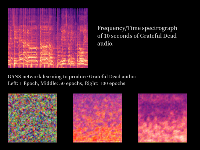
For any readers of my Grateful Dead machine-learning exploits, expect a new post in early summer.

7 years. That’s how long it took me to listen to every available Grateful Dead show.

You can view the entire list, with a mini review and my rating out of 5, here: https://raw.githubusercontent.com/maximinus/grateful-dead-reviews/master/dead_reviews.txt

It started in 2013, when I quit my teaching job and started working as a computer programmer from home, giving me the freedom to listen to music all day long. I discovered pretty quickly that this freedom brought a burden; having to choose what to play all the time. Especially since the average album only lasts for about an hour.

Luckily, I had just acquired the complete Europe 72 release, and it occured to me to voyage through it’s entirety, in sequential order. What a massive amount of Dead – it was sure to keep my ears occupied for some time! All I had to do was start the next show at the end of the current. When the supply finally ran dry, it was trivial to continue, I already a prety vast collection sat on the hard drive. I never set out to listen to every show, I was just too lazy to ever stop.

For the most part, I listened in sequential order through the dates, although I cleared different eras out of order. My journey went from 72 through 77, then back to 65 through 70. From there, I skipped to 78 and went all the way to 93. This last year or so was spent clearing up the remains and trying to make sure I hadn’t missed any shows (that Miller guy keeps dumping soundboards online).

I started to give each show a score out of 5 very early on. Maybe from the first show, but definitly from Summer 72 (I had to listen to Europe 72 twice because I lost the first scores, if they ever existed). My grades were simple, on 1 to 5 scale: 3.5 was an “average” show, going up to 5 for the very best. A score of less than 2.5 was rare, simply because there was no real need to quantitatively compare bad shows in any detail. Some shows are rated lower than 2, this is usually for those unlistenable audience tapes where the music struggles to punch through – 1970 suffers a lot from this.

Scores are of course subjective and you may disagree with what I wrote for a show. However, I would be very surprised if your favourite show scored less than 3.5. Those shows are bad on many levels. Likewise, I’d be surprised if you hated a 4.5 or upwards. I have met people whose favourite show was a 3.5.

What makes a good show? For me, above and beyond the raw music, it is a certain level of chaos, the unexpected or some deviation from the norm. For musical tastes, if a show had 1 minute of Stockhausen atonal sounds or loud feedback, that was likely half a point added. If it got emotional, that was likely another half point (like that last ever Morning Dew – “I guess it DOES matter”). Most of all, I appreciated the jamming. When the music weaved it’s own unique thread, that is when I got excited. Sometimes a majestic sonic glory of merely a few seconds could elevate a show. St Stephen intro + Mutron + loud volume – it occurs once for about 5 seconds in 78 and every single hair of mine was electrified.

But also fun were the non-musical interludes. I think of the 72 show where Wavy Gravy shares his single beer with the entire audience, the dentist’s chair in 1981, the female audience member who explains Shakedown by singing the melody line when it was a new song, the on-stage conversations – “How’s the 8-ball, Jerry?”, the audience comments – “Jerry really looks like Phil Spectre” – all of these in their own way paint a little corner of the Dead experience.

For the 1980s and onwards I mainly relied on archive.org, and reading the Deadhead stories posted there was a real delight. As the years roll on they become mere stories of excessive drug abuse (although the police dosing themselves at the penultimate show was pretty funny), but the late 70s and early 80s shows have a wealth of anecdotes, craziness and adventure. So many people with their lives changed by a random encounter with the greatest live band to ever exist. The best story was from Yugoslavian student. He studied in the early 80s in the US, and only in the last week before flying home, did he venture out with his fellow classmates for some fun. They took him to a show, fed him paper and he had an out of body religious experience with the music. Unfortunatly, upon flying home to Eastern Europe, he was unable to obtain ANY Grateful Dead until years later when the Iron curtain fell. I like to think that guy finally drank deeply from the well of tapes – after all, eventually he made it to archive.org and was able to declare his love for the band.

For the masochists out there, you’ll be wanting to hear the China Doll from 30th July 1983. Or perhaps the mystery singer who sits in for the last few songs of 8th March 1970. Or you’d just rather Jerry turned his guitar off and let someone else play, in which case Steve Miller and the Dead, post-drums on 31st May 1992 might be your particular poison. To be honest, speculating on the bad Grateful Dead is easier than the good because really, even in the depths of what we might say are the bad years, the Dead were still, on the whole, not that bad. Truly bad Dead is the inane, the boring, and if I’m honest there were only 2 periods that were a struggle: 1970, because it has so many terrible audience recordings, and 1994, because the Dead here really were at their worst.

But I’m not here to look at the worst, I’m here to celebrate the best. Having spent so much time listening, now finally I come to the project that I am really looking forward to: I am going to listen to all the good shows – some 650 of them – that rated 4 or higher. “Above average” in my parlance. Sorted randomly, not fixed by date, time. One day in the future, I will have a top 50 to recommend to you; but those will be my favourite shows, not yours. Neither of us will be right or wrong, because your relationship with the music is just as valid as mine.

The Grateful Dead then, they are a journey, an experience, a tour de force, a philosophy with the writings of Hunter. Hearing all those shows has not made me tire of the GD, it has simply propelled me to listen to the good ones again. Maybe one day I will be bored of this journey; until then, “Let there be songs – to fill the air”.